Phase 1: Photon tracing
Photon structure
Each item in our Photon class has the following components:- An
int Type, which is eitherDiffuse,Specular,Transmission, orEmitted. - Points to
Photon* PrevandPhoton* Next, which is super useful for visualizing paths and also for checking paths for caustic properties.PrevisNULLfor emitted photons. - The
RNRgb Powerof the photon. - A
R3Ray Rayshowing the starting point of the photon, and the direction its path leads in scattering. This direction isNULLfor terminal photons.
Photon emission
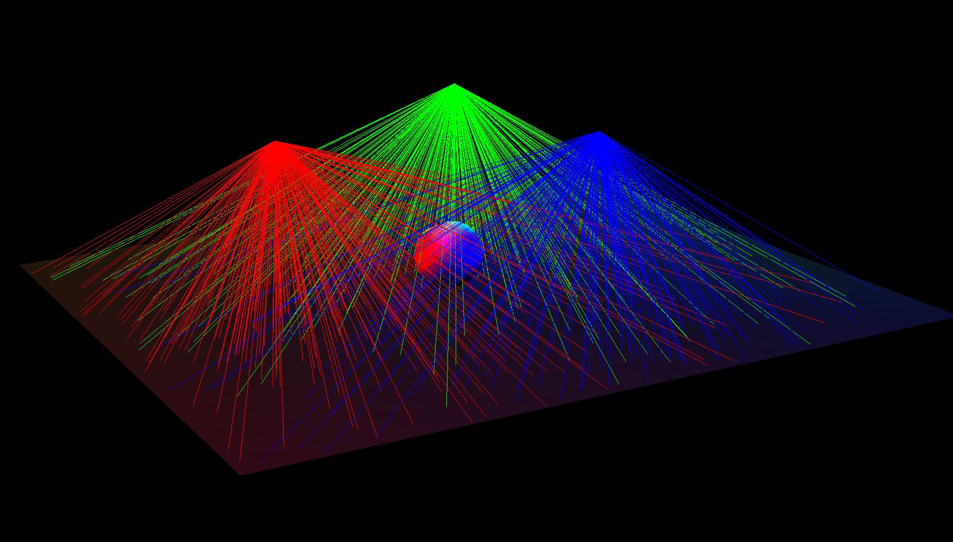
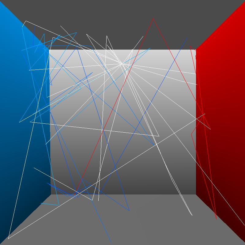
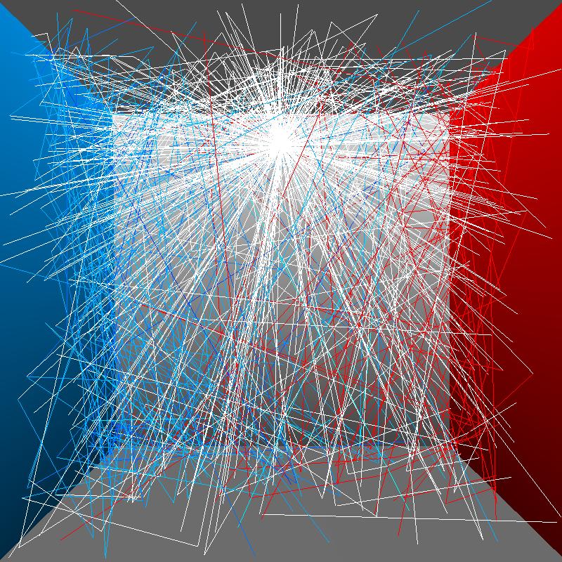
There's a hard-coded number of photons (_nTotalPhotons = 100000) that are shot out of the scene in total. What, so many photons?? If an emitted photon doesn't intersect with our scene, we don't care. It's the scene's loss! We don't replace the non-intersecting photon ray with another, which is why we emit so many to begin with. Space is not a limiting factor.
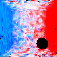
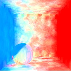
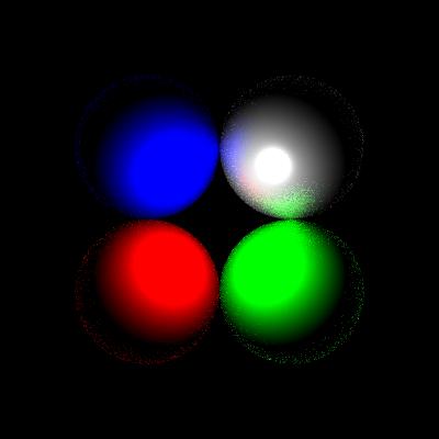
We give a proportion of these photons to each light in the scene, dependent on the light's intensity. Also, note that each photon's power is proportional to how many photons are shot out of that particular light! These emitted light visualizations have each photon's intensity as equal to the intensity of the light, so you can clearly see where photons are coming from. In implementation, however, because we're shooting many photons, each photon should carry very little power.
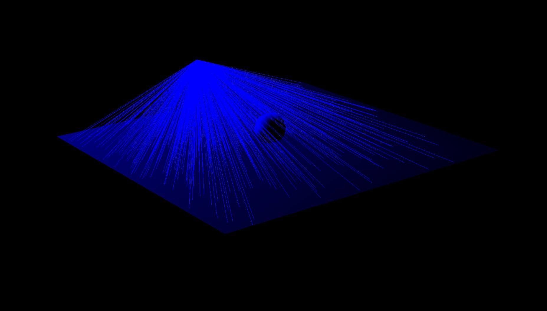
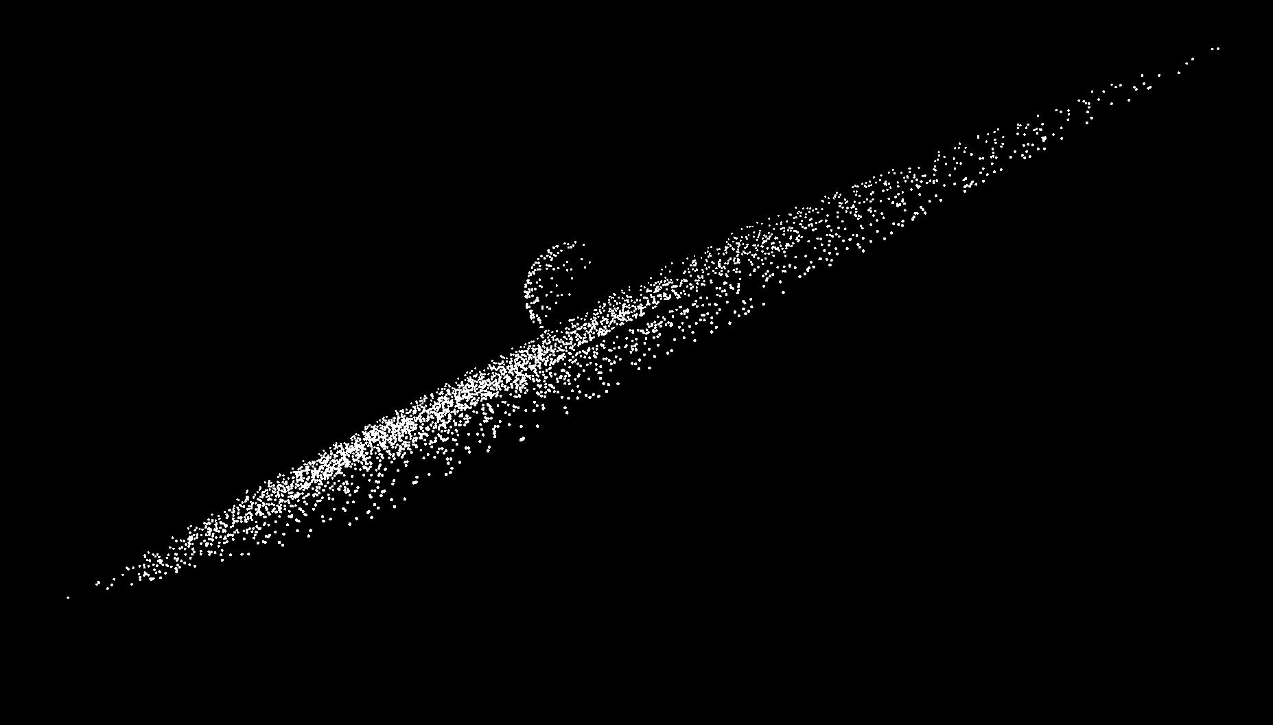
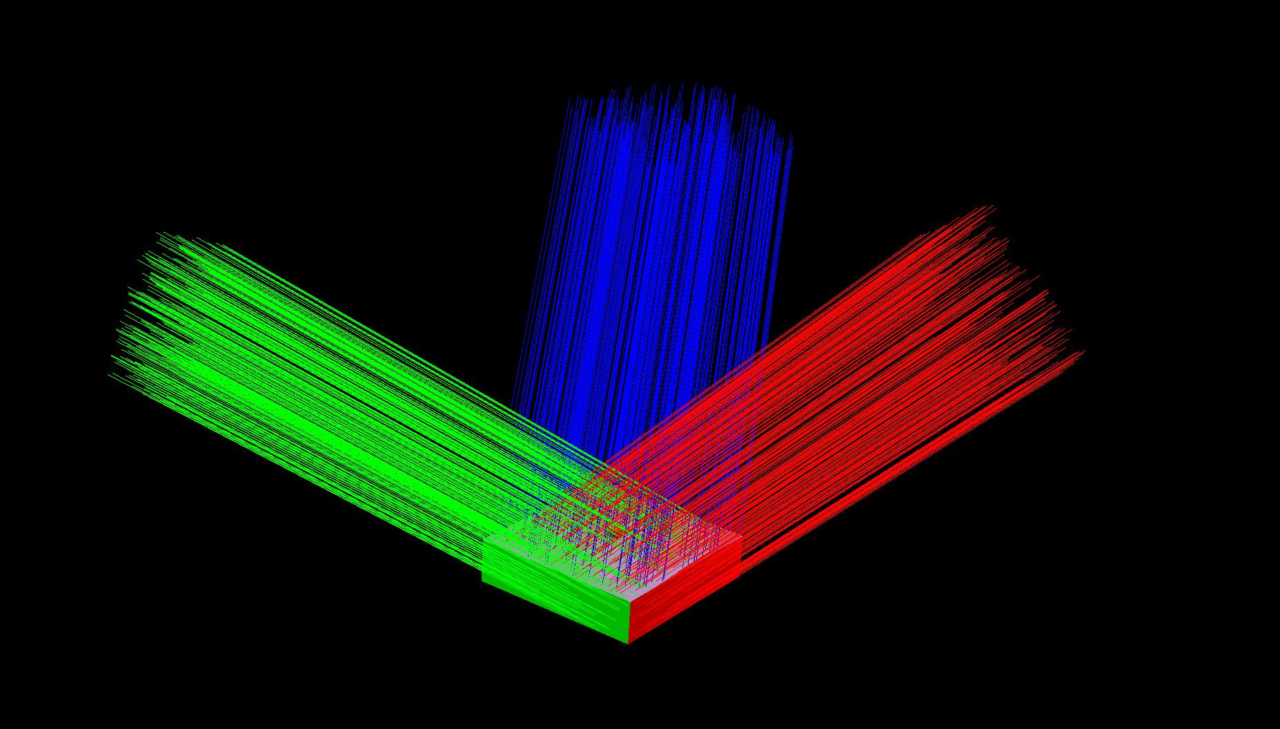
Point lights
Point lights are pretty straightforward; we position the photon at the source of the light, and emit in an arbitrary direction.
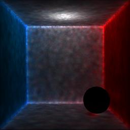
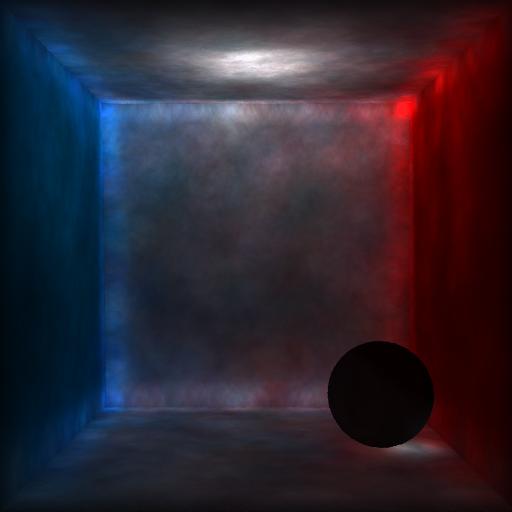
pointlight1.scn, showing paths. |
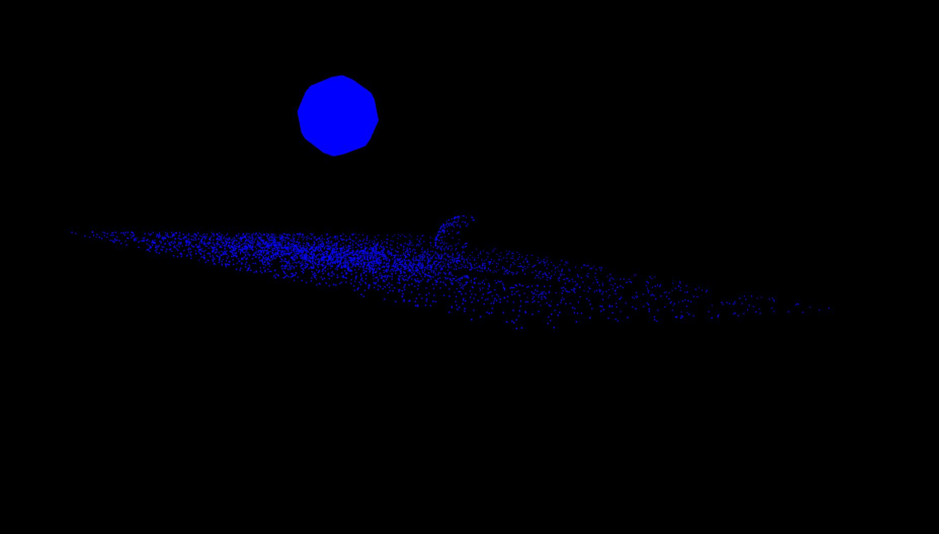
pointlight1.scn, showing photons. |
pointlight2.scn, showing paths. |
pointlight2.scn, showing photons. |
(I tried to tilt the image for points so you could see the sphere on the surface of the ground.)
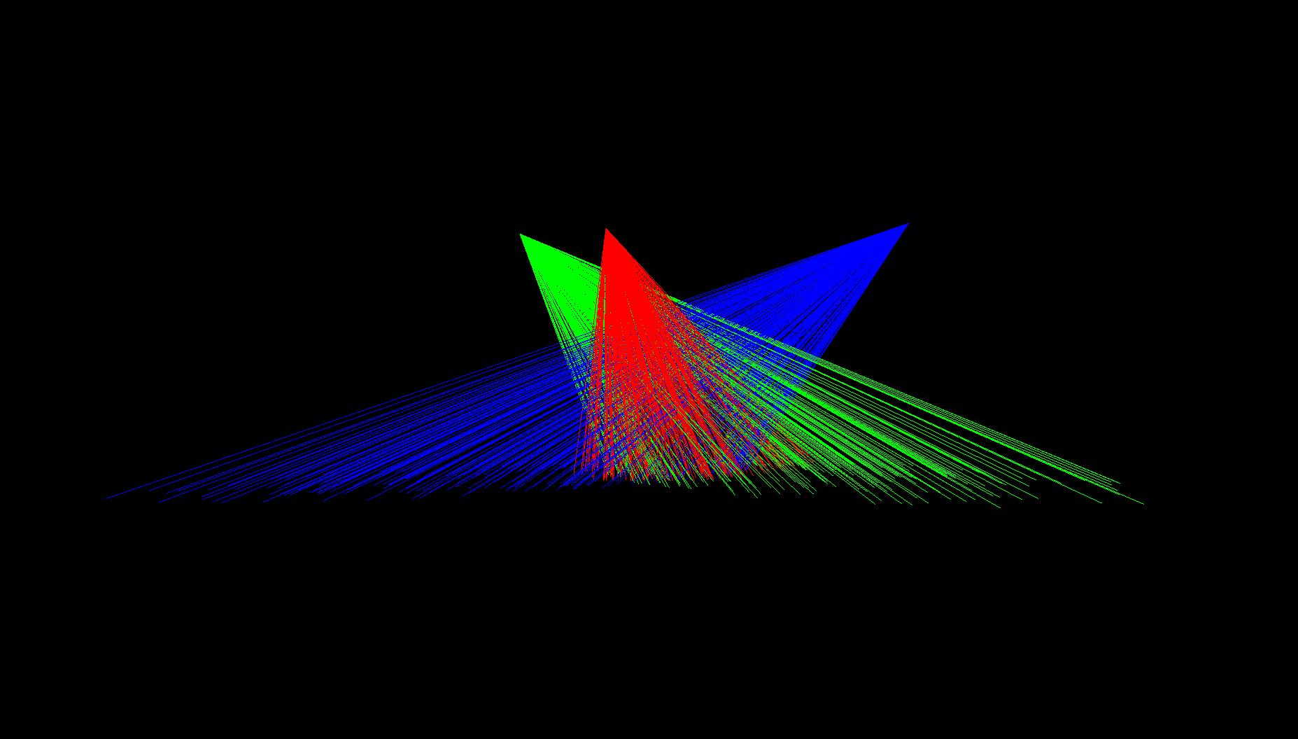
Area lights
Area lights are stored as a circle and a normal. We emit photons from randomly chosen points on the circle, in a cosine-weighted random direction (more likely to shoot in the direction of the normal).
arealight1.scn, showing paths. |
arealight1.scn, showing photons. |
arealight2.scn, showing paths. |
arealight2.scn, showing photons. |
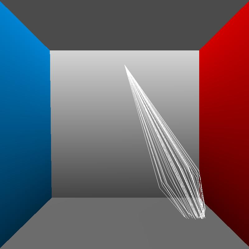
Spot lights
Spot lights are stored as a point, direction, cutoff angle, and drop off rate. We shoot photons from the spot light's origin in the hemisphere indicated by the direction, reject those that exceed the cutoff angle, and select photons randomly in proportion to a cosine/drop off rate ratio.
spotlight1.scn, showing paths. |
spotlight2.scn, showing paths. |
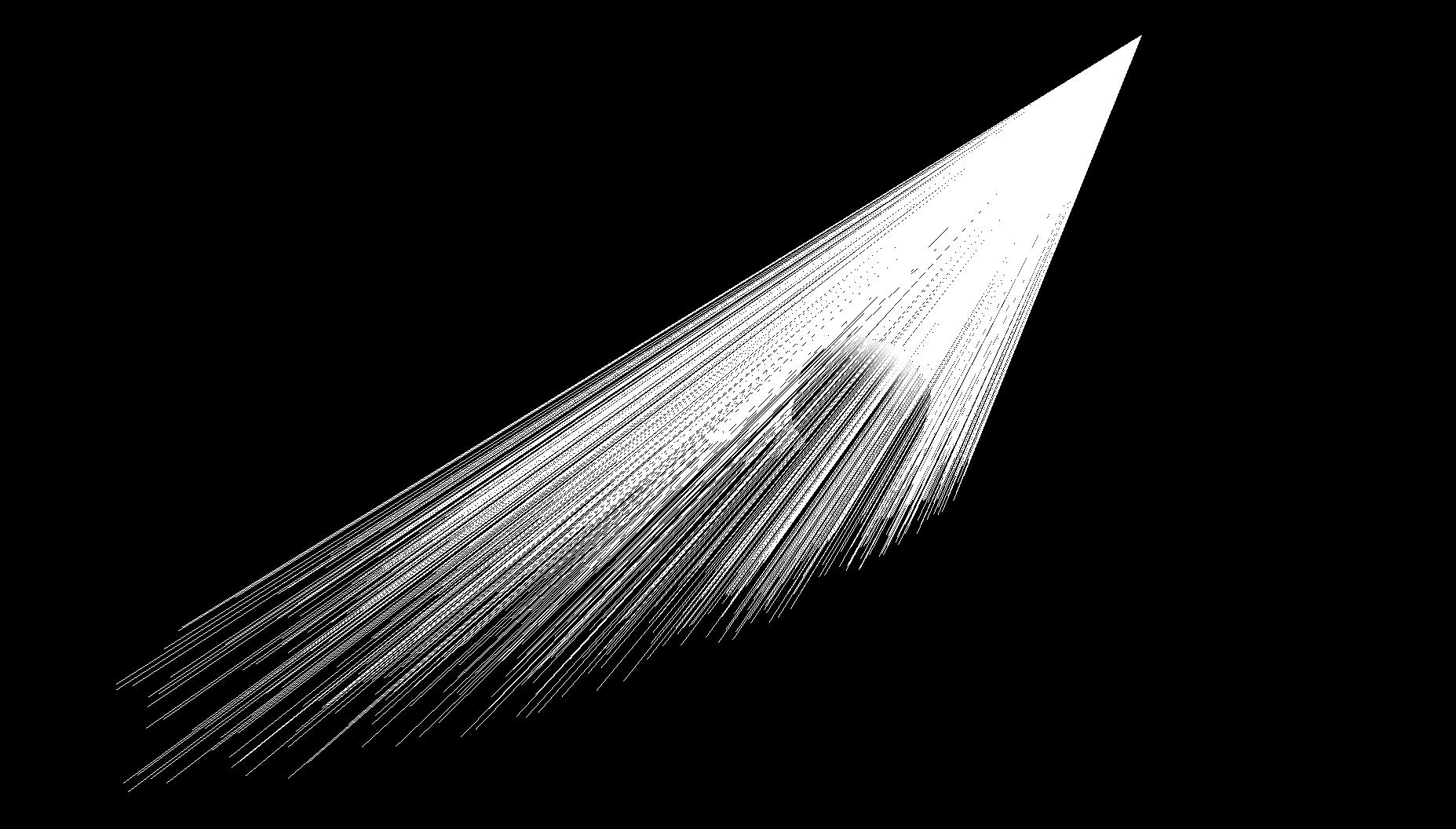
Directional lights
Directional lights are a bit difference, since they don't have a point of origin, only a direction. We make a moderately large circle outside of the bounds of the scene, and pick random points on that circle to shoot points into the specified direction. It's not specified how large of an area this directional light covers, so we arbitarily (lazily, probably) assume the area is exactly how large we make it so that our photon intensities are perfect.
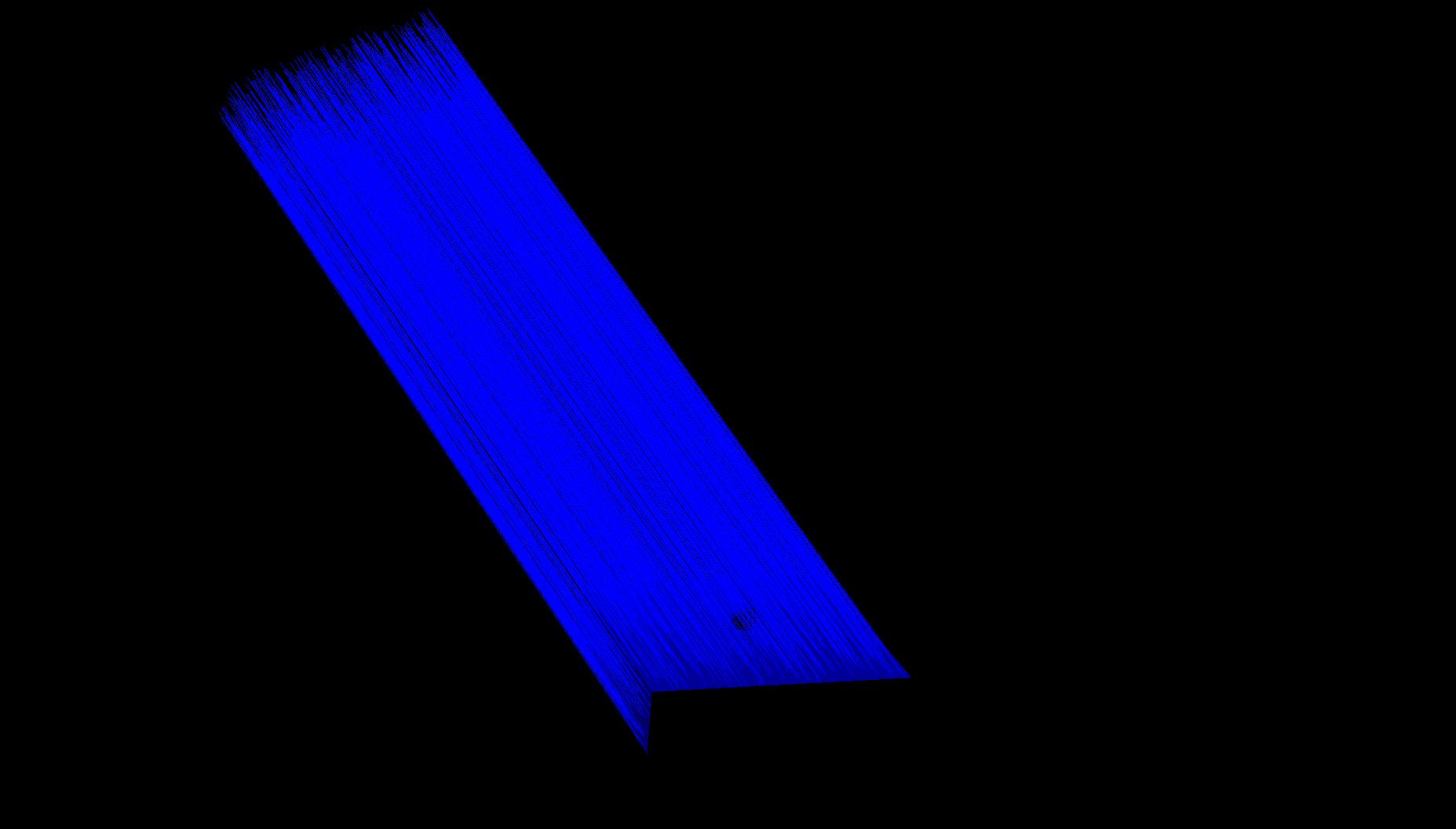
dirlight1.scn, showing paths. |
dirlight2.scn, showing paths. |
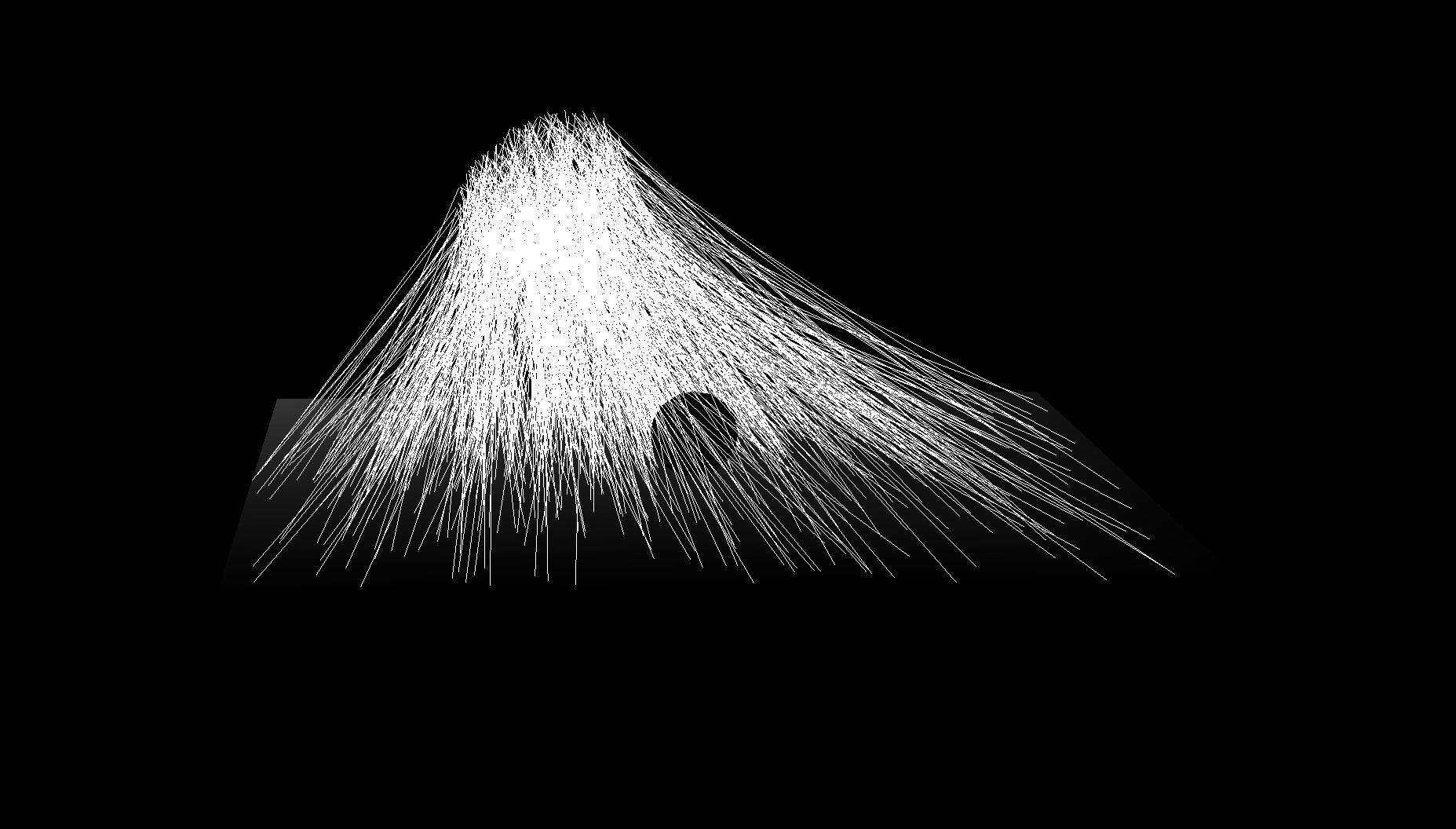
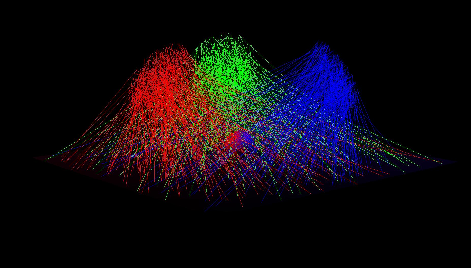
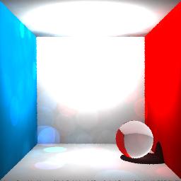
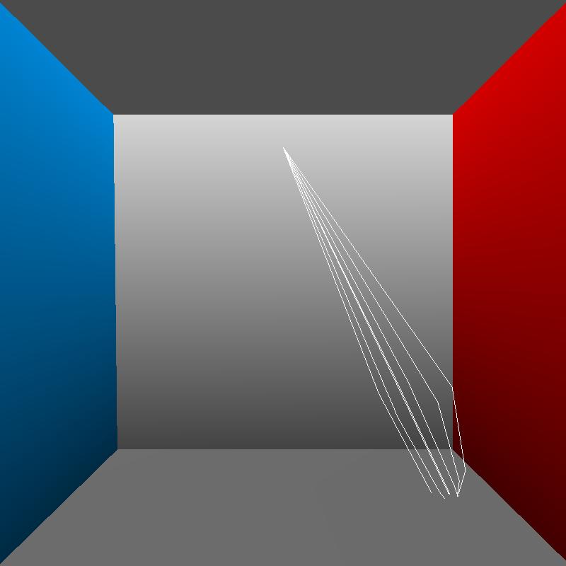
Photon scattering/ Russian Roulette/ BRDF importance sampling
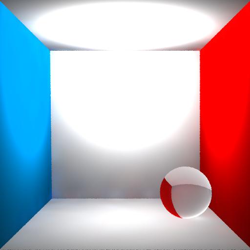
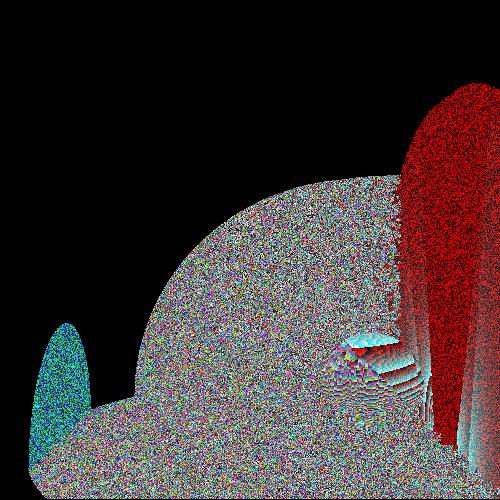
Now that we have all of these emitted photons, it's time to scatter them across the scene! (If you're following along in the code, this is my TracePhoton() function.) First, we find an intersection of the emitted photon with the scene. Depending on the brdf properties of the intersection material, there are probabilities of the path going in a diffuse, specular, or tranmission direction. Or, the path could terminate. This is Russian Roulette! My implementation gives each photon a 95% survival rate. When the photon continues, it will lose power proportional to its probability of surviving. Here are some examples of what our renderings would look like if the survival rate was lower.
|
|
If we decide that the path continues in a diffuse direction, we return a random direction along the hemisphere defined by the normal of the intersection. If the path continues in a specular direction, we choose a direction related to the shininess and angle. (Jason Lawrence's notes are really helpful here.) If the path continues in a transmission direction, based on the index of refraction and normal, we use Snell's law to get the new direction.
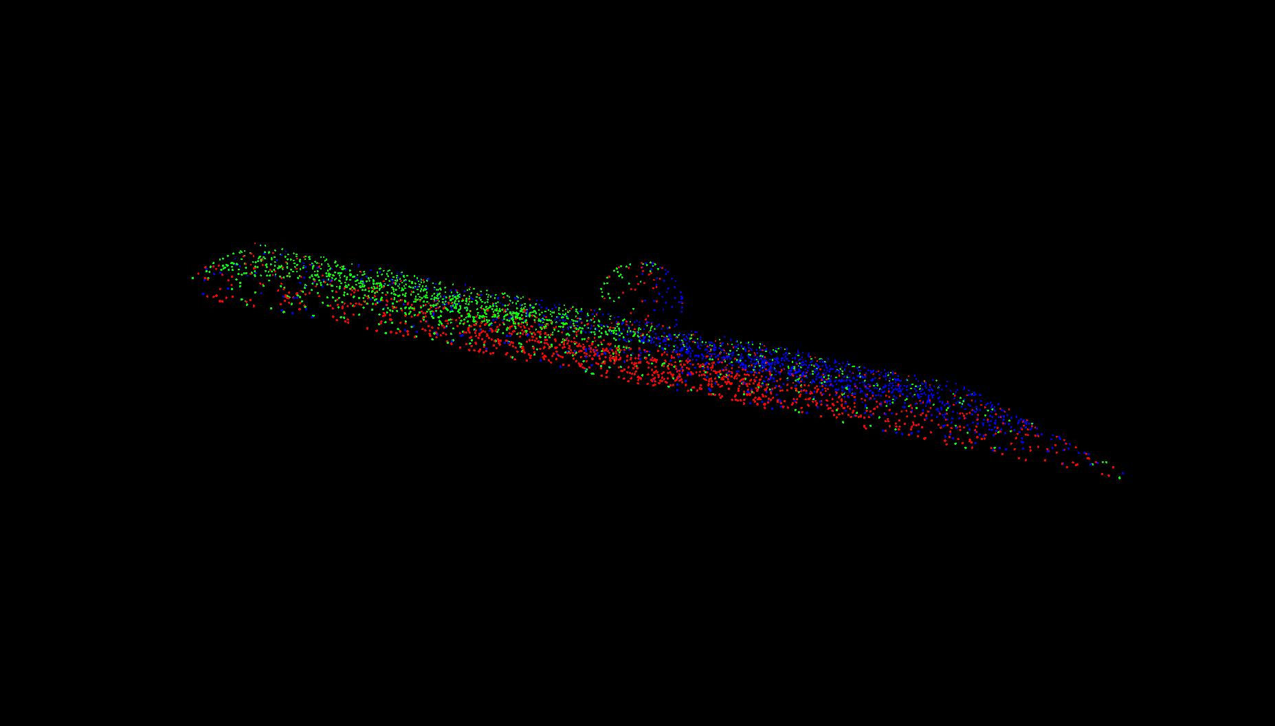
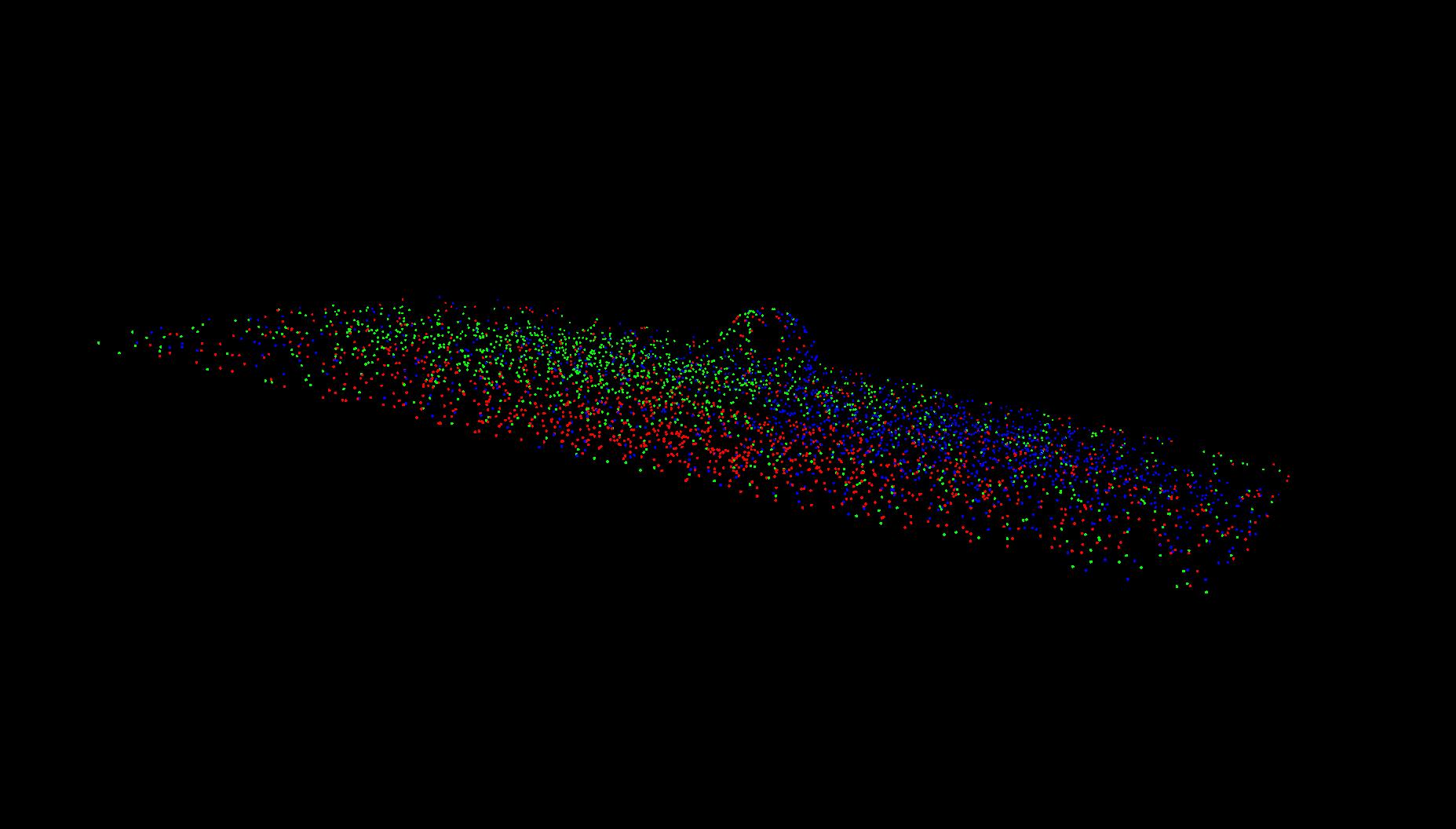
Multiple photon maps
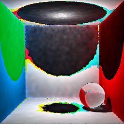
As we trace the photons, we store the diffuse photons in either a global or caustic kdtree map, based on the path the photon has traversed. If the path is from an emitted photon to a specular/transmission photon to the current diffuse photon, then we store the photon in our caustic map. If the diffuse photon took some other path, we store it in our global map. So, there are no caustic photons in the global map.
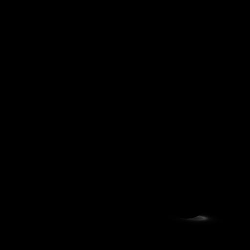
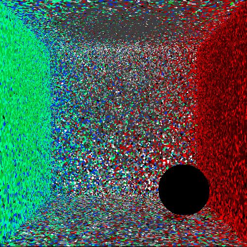
-ntotalphotons = 20). |
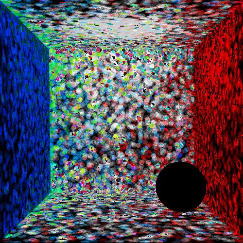
-ntotalphotons = 300). |
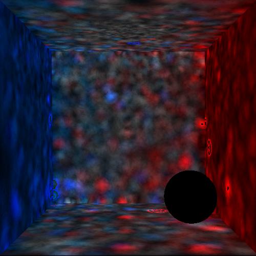
-ntotalphotons = 500). |
-ntotalphotons = 500). |
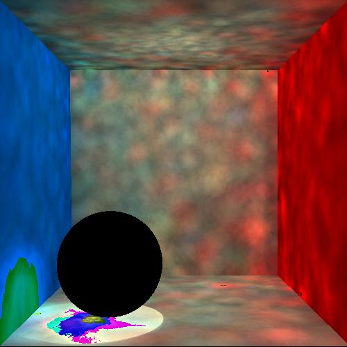
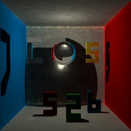
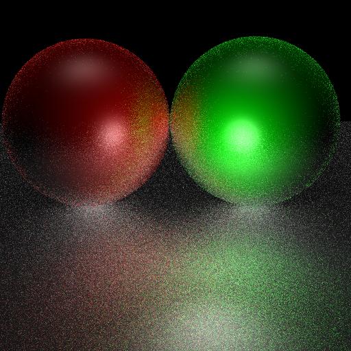
Notice that as rays bounce off the colored sides, the power changes slightly to reflect this bounce. That's why some subsequent rays are red or blue.